Inspecting the reconstruction result

The reconstruction result spring.Result is returned by the spring.MPR.run() method, which allows for an immediate inspection of the phase retrieval outcome.

However, the result is also saved on disk at the path indicated in the settings. By default, the path is set to ./, i.e. the folder where the reconstruction script was executed:

from spring import Settings
Settings().info('global','workdir')

| Section |   Name  | Value |  Type  | Range |           Description            |
| :-----: | :-----: | :---: | :----: | :---: | :------------------------------: |
|         | workdir |   ./  | string |       | Path where the results are saved |

The filename is composed by concatenating the numbers contained in the pid parameter of the pattern object with an underscore, and then adding the _rec.h5 suffix. The file is saved in HDF5 format, and can be manually loaded and inspected via the h5py python module.

However, the spring.Result class provides an interface to handle the reconstruction files in an easier way. In particular, it is possible to load a reconstruction from the storage by providing the pid (and the workdir if different from the current directory). For example:

# Get the pid of the diffraction pattern
import numpy as np

data = np.load('data/example_A_1.npz')
print(*data['pid'])

# Load the reconstruction
from spring import Result
rec = Result(data['pid'])

197 10 14558540587

It is possible to see how the filename is formatted by using the spring.Result.get_filename method of a reconstruction:

print(Result().get_filename(pid=data['pid']))
print(Result().get_filename(pid=[123,456789], tag='test1'))

197_10_14558540587_rec.h5
123_456789_test1_rec.h5

The filename can be then also manually specified using the spring.Result.loadfile method and indicating the full path to the file, i.e.:

rec_manual = Result().loadfile('./197_10_14558540587_rec.h5')

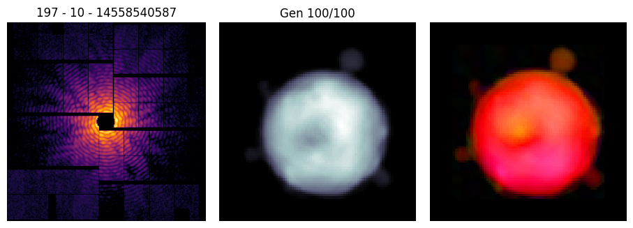
The quickest way to get an overview on the result is to call the spring.Result.plot() method

rec.plot()

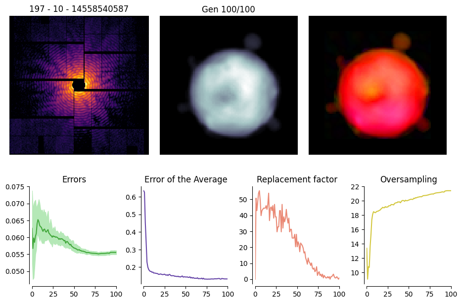
Further information can be gained by adding the stats=True option, which reports the behavior of some performance indicators along the reconstruction process

rec.plot(stats=True)

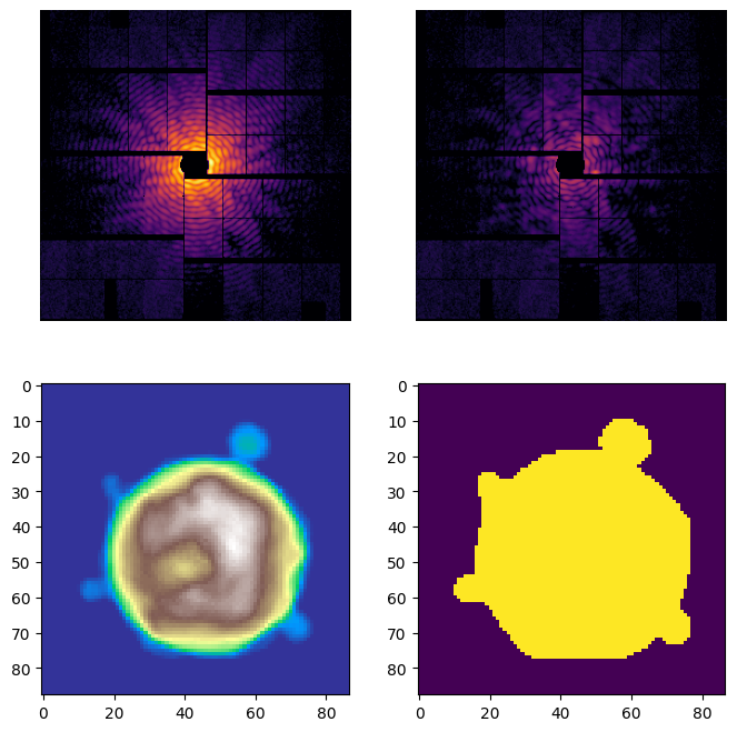
It is possible to manually fill a plot with a custom layout and a custom content, for example in the following way:

import matplotlib.pyplot as plt

fig, ax = plt.subplots(2,2, figsize=(8,8))
rec.plot_pattern(ax[0][0])
rec.plot_residuals(ax[0][1])
rec.plot_density(ax[1][0], cmap='terrain')
rec.plot_support(ax[1][1])
ax[1][0].axis('on')
ax[1][1].axis('on')
plt.show()